tXploreR

Evaluating the treatment effects at each individual trial site (sub-field analysis) and across sites (cross-site analysis): An example of end-to-end analyses

Fig: Data workflow chart to demonstrate data ingestion, data analysis, and result reporting

Methods:

At first, data schema for the observed and analyzed data were created in MySQL. Data schema were created based on the column headers from the observed data (i.e. the provided data). For saving the relevant information from the analyses, I decided to store average effect of the treatments per site for both the traits in the data table "analyzed_data". This table will be generated as a part of the analyses and will be ingested into the MySQL database ("indigo_dev").

Data schema was written and ran in MySQL server. Observed data was also ingested to database via MySQL server.

-- Step 1: creating the database
CREATE DATABASE indigo_dev;


-- Before creating tables, make sure the database exists using Step 1
-- Step 2: Create table/schema for observed data


CREATE TABLE indigo_dev.observed_data (
    observed_id INT NOT NULL AUTO_INCREMENT,
    site VARCHAR(10) NOT NULL,
    row_no INT,
    column_no INT,
    rep_no INT,
    plot_no INT NOT NULL,
    treatment_no VARCHAR(10) NOT NULL,
    trait1 INT,
    trait2 INT,
    created_dt DATETIME DEFAULT NOW(),
    PRIMARY KEY (observed_id),
    UNIQUE KEY unique_obs (site,plot_no)
);

-- Add index on treatment
ALTER TABLE indigo_dev.observed_data ADD INDEX treatment_idx(treatment_no);

-- Step 3: Create table/schema for analyzed data
CREATE TABLE indigo_dev.analyzed_data (
    analyzed_id INT NOT NULL AUTO_INCREMENT,
    treatment_no VARCHAR(10) NOT NULL,
    rep_count INT,
    measurement_mean FLOAT,
    measurement_std FLOAT,
    site VARCHAR(10) NOT NULL,
    trait VARCHAR(10) NOT NULL,
    created_dt DATETIME DEFAULT NOW(),
    PRIMARY KEY (analyzed_id),
    UNIQUE KEY unique_anlyz (site,trait,treatment_no) ,
    CONSTRAINT FK_site FOREIGN KEY (site) REFERENCES indigo_dev.observed_data(site),
    CONSTRAINT FK_treatment FOREIGN KEY (treatment_no) REFERENCES indigo_dev.observed_data(treatment_no)
    )
    ;


---### INGESTION ###

-- Loading observed data
SET GLOBAL local_infile=true;

LOAD DATA LOCAL INFILE '/Users/admin/Desktop/indigo/observed_data.csv'
INTO TABLE indigo_dev.observed_data
FIELDS TERMINATED BY ','
LINES TERMINATED BY '\n'
IGNORE 1 ROWS
(site,row_no,column_no,rep_no,plot_no,treatment_no,trait1,trait2);
  

ER model to show how to organize the observed and analyzed data

Now I have created a MySQL database, I will be extracting table (observed_data) from the database and use it to make statistical models. Model building and comparisons will be mostly done in R using variuos statistical packages.

# loading packages
library(RMySQL)
library(effects)
library(broom)
library(tidyverse)
library(multcomp)
library(lme4)
library(nlme)
  

Read in data from MySQL database.

# Read in data from MySQL database

con_sql <- dbConnect(RMySQL::MySQL(), group = "indigo_dev")

## .my.cnf file saved in `~/.my.cnf ` with credentials
## [indigo_dev] database=indigo_dev user=root port=3306
## password=root host=127.0.0.1

# table
observed_data <- dbReadTable(conn = con_sql, name = "observed_data")

# convert into factor
observed_data$site <- as.factor(observed_data$site)
observed_data$treatment_no <- as.factor(observed_data$treatment_no)

# make wide data table to long format- as long format is
# more suitable for subsetting.
d_long <- gather(observed_data, Trait, measurement, trait1:trait2,
    factor_key = TRUE)
  

Now I have processed the observed data and is ready to be used in model bulding part. For this data, we have two traits (reponse variables). We need to compare the effectiveness of the microbial seed-coating in two study sites (Site1 and Site2), as well as in overall-sites. When we compared the means, we use one-way ANOVA for model building. Post-hoc test for pairwise mean comparisons was performed with Tukey's method at alpha 0.05. For each trait, we need to build 3 models:

For Site 1 - Here we are using linear model.
For Site 2 - Here we are using linear model.
For Overall Sites - for overall sites, we need to consider sites as a block and pass as a random factor in Linear Mixed Model.

First, lets summarized the means and ingest the results to our MySQL database.

# Function to get summary about trait at each site by
# treatments.
get_summary_by_sites_and_trait <- function(data = d_long, site = s,
    trait = t) {
    # subset data
    d_st <- data %>%
        filter(site == site & Trait == trait)

    # summary
    summary_df <- group_by(d_st, treatment_no) %>%
        summarise(count = n(), mean = mean(measurement, na.rm = TRUE),
            sd = sd(measurement, na.rm = TRUE))

    summary_df <- data.frame(summary_df)
    summary_df["site"] <- site
    summary_df["trait"] <- trait
    summary_df
}
  

# Run the above function to each site and trait combination
summary_s1_t1 <- get_summary_by_sites_and_trait(data = d_long,
    site = "Site1", trait = "trait1")
summary_s1_t2 <- get_summary_by_sites_and_trait(data = d_long,
    site = "Site1", trait = "trait2")
summary_s2_t1 <- get_summary_by_sites_and_trait(data = d_long,
    site = "Site2", trait = "trait1")
summary_s2_t2 <- get_summary_by_sites_and_trait(data = d_long,
    site = "Site2", trait = "trait2")

# bind multiple data frames to one
analyzed_data <- rbind(summary_s1_t1, summary_s1_t2, summary_s2_t1,
    summary_s2_t2)

# Rename column – with more information, and matches with
# data schema in the MySQL database.
colnames(analyzed_data) <- c("treatment_no", "rep_count", "measurement_mean",
    "measurement_std", "site", "trait")

head(analyzed_data)
  

##   treatment_no rep_count measurement_mean measurement_std  site  trait
## 1      Control         8          2388438        264342.0 Site1 trait1
## 2         Trt1         8          2593973        724682.5 Site1 trait1
## 3         Trt2         8          2688393        438029.1 Site1 trait1
## 4         Trt3         8          2111384        549891.4 Site1 trait1
## 5         Trt4         8          2451339        677581.7 Site1 trait1
## 6         Trt5         8          2845759        423212.6 Site1 trait1
  

Data ingestion to MySQL database.

Now we can ingest the analyzed data table to indigo_dev database.

## Table is already created, just appending values, instead
## of overwriting

dbWriteTable(conn = con_sql, name = "analyzed_data", value = analyzed_data,
    append = TRUE, row.names = FALSE)
  

## [1] TRUE

# check the ingested tables
dbListTables(conn = con_sql)
  

## [1] "analyzed_data" "observed_data"

Function to run models by trait. This function runs three models for each trait.

Linear model for Site1
Linear model for Site1
Mixed model, where Sites (block) are considered as random factor

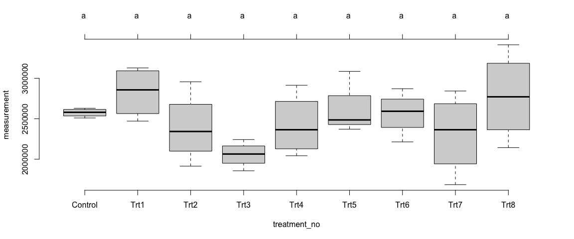
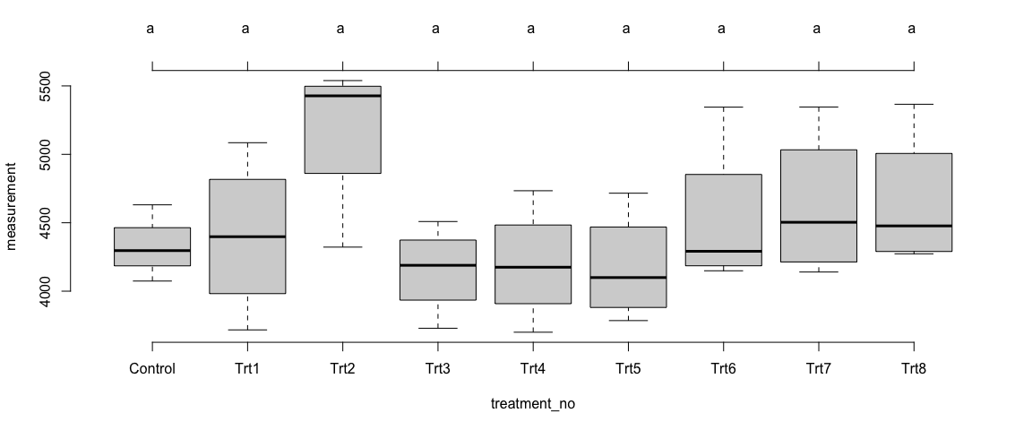
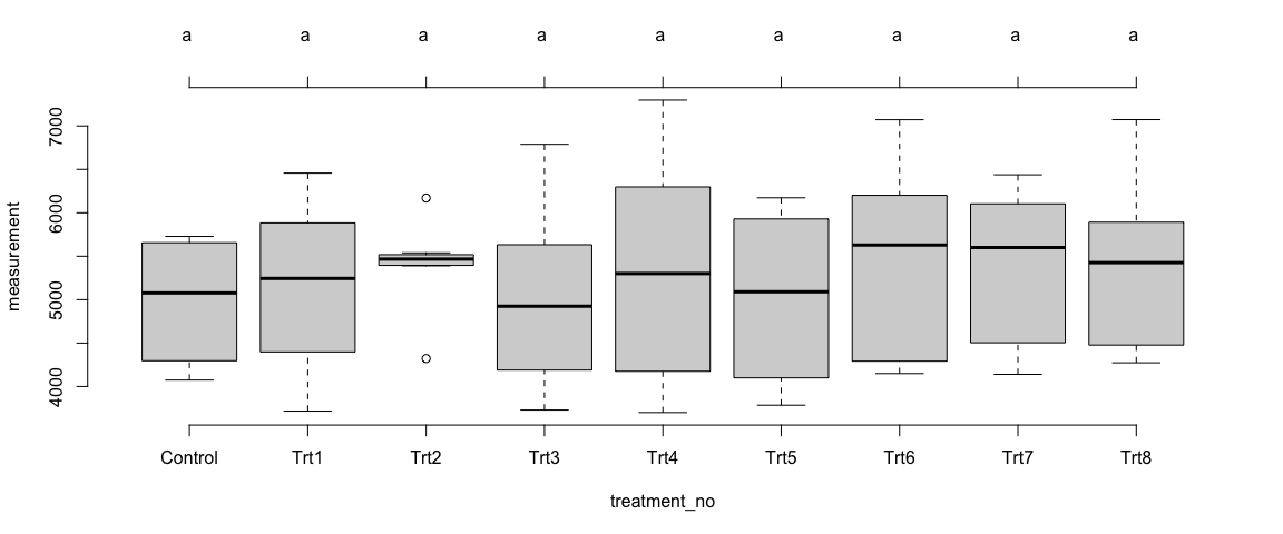
Multiple outputs from each model are embedded as a nested list object, which can be called to compare tables/outputs from the model-run or plot the boxplot. Multiple pairwise comparisons of means are summarized by letters at the top of the boxplot. Boxplot not sharing the same alphabet indicates the statistical evidence (p<0.05) for the differences in the trait means. If the letter is the same across the boxplot, then it means there is lack of strong evidence (p > 0.05) to support the differences in the trait means.

# rather than copying and pasting code for multiple times,
# creating a functions make more sense here. Function takes
# in data and trait #information, then build three models
# as described above.

run_model_by_trait <- function(data, trait) {

    # subset data
    d_t <- data %>%
        filter(Trait == trait)

    # Comparisons of treatment within a location.  site1
    d_t_s1 <- d_t %>%
        filter(site == "Site1")

    # model_list_object
    model_lst_obj_s1 <- list()

    # model
    model_t_s1 <- lm(measurement ~ treatment_no, data = d_t_s1)
    model_lst_obj_s1[[1]] <- model_t_s1
    model_lst_obj_s1[[2]] <- anova(model_t_s1)
    model_lst_obj_s1[[3]] <- tidy(model_t_s1, effects = "fixed",
        conf.int = TRUE)
    model_lst_obj_s1[[4]] <- augment(model_t_s1, d_t_s1, interval = "confidence")
    model_lst_obj_s1[[5]] <- confint(glht(model_t_s1, linfct = mcp(treatment_no = "Tukey")))
    model_lst_obj_s1[[6]] <- cld(model_lst_obj_s1[[5]])  # compact letter declaration
    names(model_lst_obj_s1) <- c("model", "ANOVA", "tidyOutput",
        "AugmentOutput", "AllpairComp", "tuk-cld")
    model_lst_obj_s1

    d_t_s2 <- d_t %>%
        filter(site == "Site2")

    # model_list_object
    model_lst_obj_s2 <- list()

    # model
    model_t_s2 <- lm(measurement ~ treatment_no, data = d_t_s2)
    model_lst_obj_s2[[1]] <- model_t_s2
    model_lst_obj_s2[[2]] <- anova(model_t_s2)
    model_lst_obj_s2[[3]] <- tidy(model_t_s2, effects = "fixed",
        conf.int = TRUE)
    model_lst_obj_s2[[4]] <- augment(model_t_s2, d_t_s2, interval = "confidence")
    model_lst_obj_s2[[5]] <- confint(glht(model_t_s2, linfct = mcp(treatment_no = "Tukey")))
    model_lst_obj_s2[[6]] <- cld(model_lst_obj_s2[[5]])  # compact letter declaration
    names(model_lst_obj_s2) <- c("model", "ANOVA", "tidyOutput",
        "AugmentOutput", "AllpairComp", "tuk-cld")
    model_lst_obj_s2

    # model_list_object
    model_lst_obj_s3 <- list()

    # model 3 where sites is treted as random factor --
    # block
    model_t <- lme(measurement ~ treatment_no, random = ~1 |
        site, d_t, method = "REML")
    model_lst_obj_s3[[1]] <- model_t
    model_lst_obj_s3[[2]] <- anova(model_t)
    model_lst_obj_s3[[3]] <- confint(glht(model_t, linfct = mcp(treatment_no = "Tukey")))
    model_lst_obj_s3[[4]] <- cld(model_lst_obj_s3[[3]])  # compact letter declaration
    names(model_lst_obj_s3) <- c("model", "ANOVA", "AllpairComp",
        "tuk-cld")

    final_list <- list(model_lst_obj_s1, model_lst_obj_s2, model_lst_obj_s3)
    names(final_list) <- c("Model_Site1", "Model_Site2", "OverallSites_MixModel")
    final_list
}
  

Analyses for Trait1

Trait1 <- run_model_by_trait(data = d_long, trait = "trait1")
names(Trait1)
  

## [1] "Model_Site1"           "Model_Site2"           "OverallSites_MixModel"

Trait 1 - Site 1

# Check model fit
par(mfrow = c(2, 2))
plot(Trait1$Model_Site1$model)
  

Mean comparision among treatments

plot(Trait1$Model_Site1$`tuk-cld`, frame.plot = F)
  

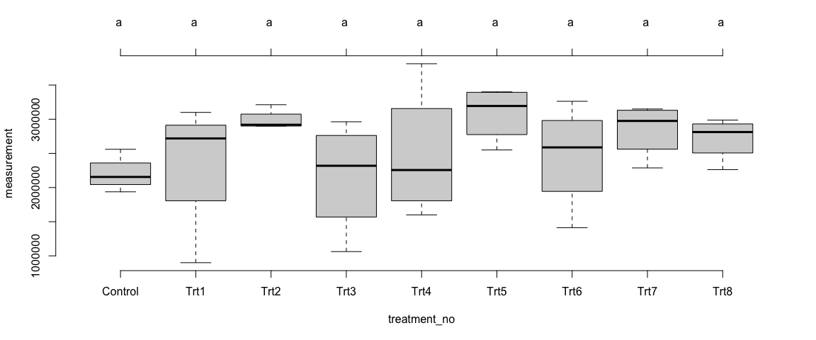
Trait 1 - Site 2

# Check model fit
par(mfrow = c(2, 2))
plot(Trait1$Model_Site2$model)
  

### Mean comparision among treatments

plot(Trait1$Model_Site2$`tuk-cld`, frame.plot = F)
  

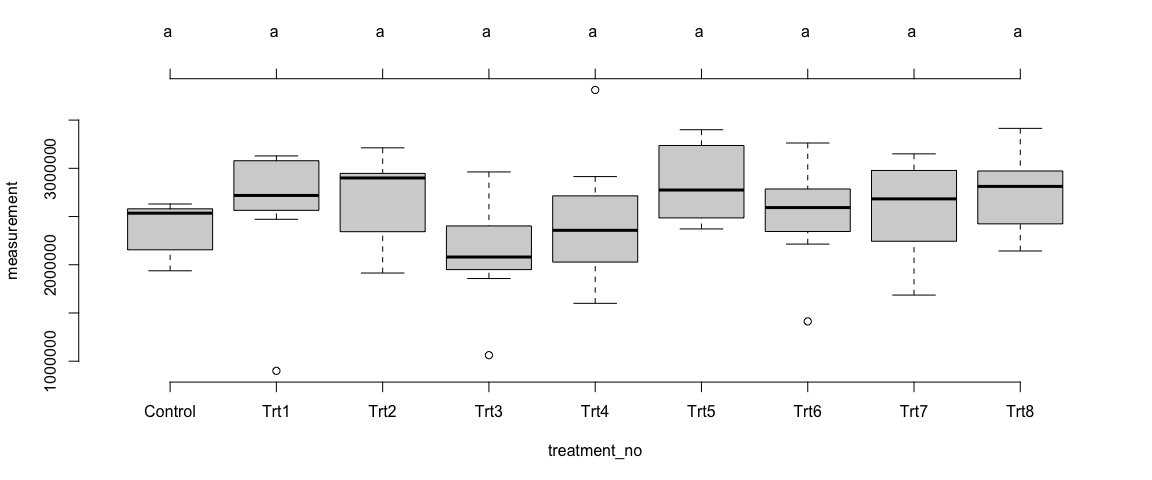
Trait 1 - Overall Sites

# Check model fit par(mfrow=c(2,2)) plot(Trait1$OverallSites_MixModel$model)
qqnorm(resid(Trait1$OverallSites_MixModel$model))
qqline(resid(Trait1$OverallSites_MixModel$model))
  

Mean comparision among treatments

plot(Trait1$OverallSites_MixModel$`tuk-cld`, frame.plot = F)
  

Summary of Results:

We observed differences in the means of trait1 across the treatments – at the individual sites as well as in overall sites. The differences among the treatments were not statistically significant (p>0.05).

Analyses for Trait2.

Trait2 <- run_model_by_trait(data = d_long, trait = "trait2")
names(Trait2)
  

## [1] "Model_Site1"           "Model_Site2"           "OverallSites_MixModel"

## list within a list object
names(Trait2$Model_Site1)
  

## [1] "model"         "ANOVA"         "tidyOutput"    "AugmentOutput" "AllpairComp"   "tuk-cld"
  

# If we need to see ANOVA table
Trait2$Model_Site1$ANOVA
  

## Analysis of Variance Table
## 
## Response: measurement
##              Df  Sum Sq Mean Sq F value Pr(>F)
## treatment_no  8 2588066  323508   1.415 0.2352
## Residuals    27 6172971  228629
  

# Site 2 ANOVA table
Trait2$Model_Site2$ANOVA
  

## Analysis of Variance Table
## 
## Response: measurement
##              Df  Sum Sq Mean Sq F value Pr(>F)
## treatment_no  8 3393794  424224  1.8917 0.1031
## Residuals    27 6055030  224260
  

# Overall sites ANOVA table
Trait2$OverallSites_MixModel$ANOVA
  

##              numDF denDF  F-value p-value
## (Intercept)      1    62 47.31872  <.0001
## treatment_no     8    62  1.09259  0.3805
  

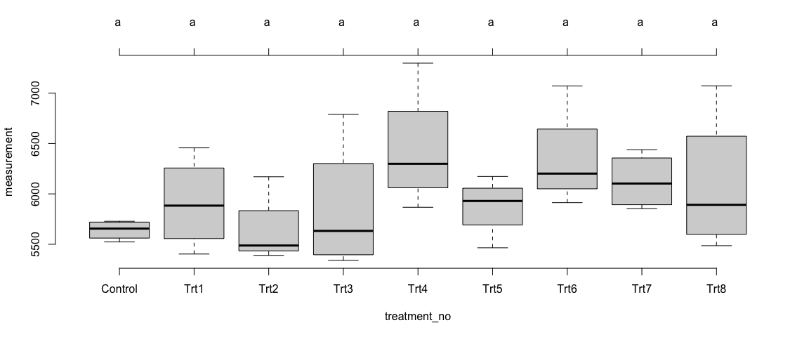
Trait 2 - Site 1

# Check model fit
par(mfrow = c(2, 2))
plot(Trait2$Model_Site1$model)
  

Mean comparision among treatments

plot(Trait2$Model_Site1$`tuk-cld`, frame.plot = F)
  

Trait 2 - Site 2

# Check model fit
par(mfrow = c(2, 2))
plot(Trait2$Model_Site2$model)
  

### Mean comparision among treatments

plot(Trait2$Model_Site2$`tuk-cld`, frame.plot = F)
  

Trait 2 - Overall Sites

# Check model fit par(mfrow=c(2,2)) plot(Trait1$OverallSites_MixModel$model)
qqnorm(resid(Trait2$OverallSites_MixModel$model))
qqline(resid(Trait2$OverallSites_MixModel$model))
  

Mean comparision among treatments

plot(Trait2$OverallSites_MixModel$`tuk-cld`, frame.plot = F)
  

Summary of Results:

Like the trait1, we observed some differences in the means of trait2 across the treatments – at the individual sites as well as in overall sites. However, the differences among the treatments were not statistically significant (p>0.05).

Shiny App

Link to the shiny app tXploreR